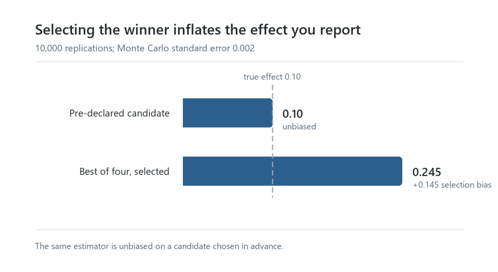
Pick the best of four prompt variants on a 50-item eval. The true improvement is 10 points. You will report 24.5.
That is not a hypothetical. It is a measured result from this library’s validation suite, run over 10,000 replications: selection bias of 0.145 on a true effect of 0.10, with a Monte Carlo standard error of 0.002. The same estimator applied to a pre-declared candidate is unbiased. The inflation comes entirely from picking the winner.
Most teams shipping LLM features are running experiments with no experimental design. They change a prompt, see a 4% improvement on fifty examples, and ship it. There is no power analysis, no confidence interval, no correction for having tested six variants, and no check on whether the LLM judge scoring the outputs prefers whichever response was listed second.
I built a library that fixes this, and I validated it by simulation rather than by assertion.
What it does
Inference that matches the data. Eval comparisons are paired and usually clustered — several questions drawn from one document are not independent. The library reduces every comparison scenario to item-level differences and runs one inference engine over them: a cluster percentile bootstrap for intervals and a cluster sign-flip permutation test for p-values, with exact enumeration below 13 clusters and an analytic cluster-robust interval as a cross-check. Classical tests appear as identity checks: sign-flip on binary singletons must reproduce McNemar’s exact distribution, and the validation suite asserts it.
Power analysis before you spend. Given your variance and the effect you care about, how many items do you need? Run it in reverse and the answer is uncomfortable: a 50-item binary eval cannot detect a difference below roughly 21 percentage points. Most teams have never computed this number for their own eval.
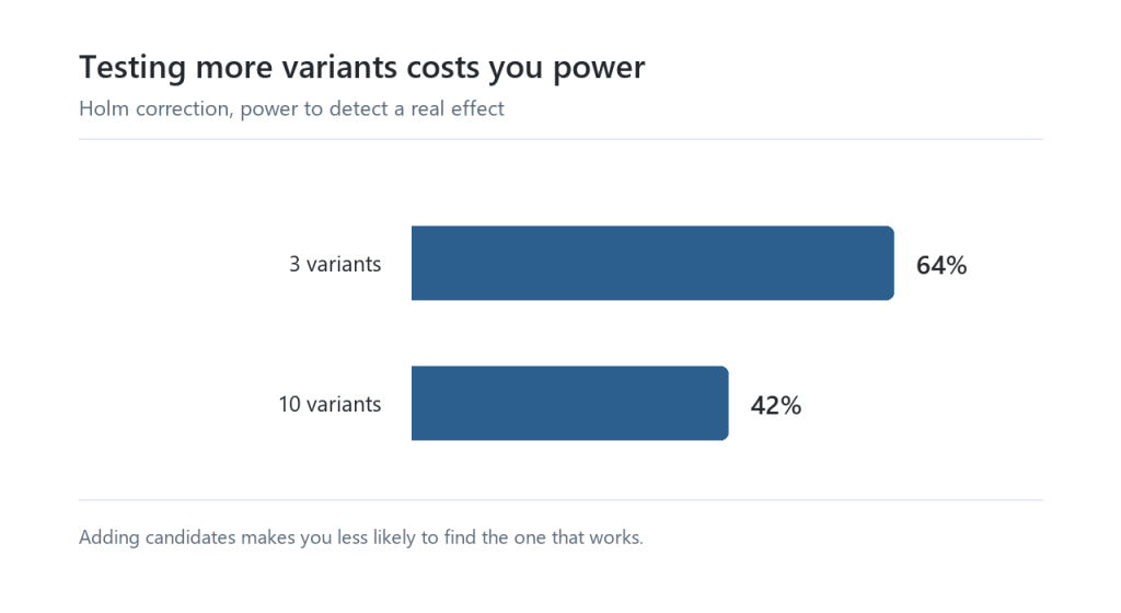
Multiplicity, and what it costs. Testing more variants is not free. Holm correction at three variants gives 64% power on a real effect. At ten variants, 42%. Adding candidates makes you less likely to find the one that works.
Judge bias, measured rather than assumed. Counterbalancing is structural in the data model: every pairwise comparison is judged in both presentation orders, and verdicts are recorded as first-or-second rather than as which variant won, so the raw observation survives for analysis. Position bias is the additive order effect. Self-preference is a cross-judge contrast, which separates a judge favoring its own outputs from those outputs actually being better — in validation, a third of the apparent self-preference was genuine quality.
Verbosity bias is not identified from observational data, and the library says so. The quantity people want is causal: the effect of length with quality held fixed. What you can observe is the association between length and preference. Nothing in a judgment record separates them — there is no quality covariate, conditioning on the judge’s own verdict is circular, and every available instrument for length also moves quality directly. In simulation, 44% of the apparent effect was confound. So the library reports a labeled association, never named as bias, alongside a controlled-manipulation estimator that only accepts data from a designed study — and that estimator reports its padding and condensing arms separately, because their difference is a check on whether the manipulation preserved quality. In one validation cell the pooled estimate reads a perfectly plausible 0.09 while the two arms sit at 0.05 and 0.13. The pooled number hides a contaminated manipulation. Only the split reveals it.
How correctness was established
Unit tests check that a function returns the right shape. They cannot tell you a bootstrap interval is a 95% interval.
Every estimator in this library has a simulation study behind it, run at 10,000 replications, with published result tables in the repository. Interval coverage is measured against nominal. False positive rate is measured under a true null. Empirical power is checked against the analytic power function. FWER and FDR control are verified at three, five, and ten hypotheses. Undercoverage and anti-conservatism fail the build; conservatism is recorded and reported.
The full suite reproduces exactly across runs. Only tables whose code changed show a diff.
What it gets wrong
The percentile bootstrap undercovers at small cluster counts. Measured: 92.6% coverage at 20 clusters against a nominal 95%, rising to 94.2% at 50 and 94.7% at 200. The shortfall is about eleven standard errors at 10,000 replications, and it replicates across roughly twenty independent estimator cells. It is a property of the resampling method, not of any one estimand.
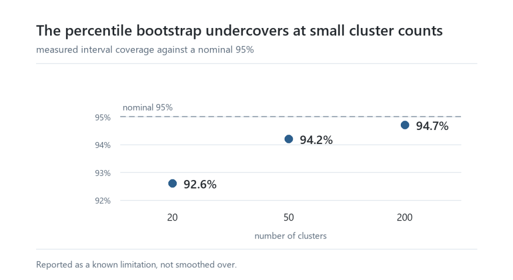
The library therefore reports the analytic interval as primary below a threshold cluster count, and discloses measured coverage in the report block rather than letting a user assume their 95% interval is 95%.
One-sided permutation tests carry a level error when the null differences are asymmetric — a nominal 5% test measured at 9.1% in the worst cell at 20 clusters. Exact binary tests are conservative by discreteness, at 2.7% against a nominal 5%, which costs real power. Both are documented, both were predicted analytically before being measured, and both are in the repository’s known-limitations section.
Publishing your own failure modes is not a disclaimer. On a project about honest measurement it is the argument.
A position bias study
I used the library to run a pre-registered study on the judges themselves: 300 prompts sampled from Arena-Hard-Auto at a pinned revision, two response pairs per prompt, every pair judged in both presentation orders by Claude Opus 5, Sonnet 5, and Haiku 4.5. 3,960 judge calls. The design, the falsification criteria, and the analysis were committed to the repository before the first API call.
Judges prefer whatever is shown second
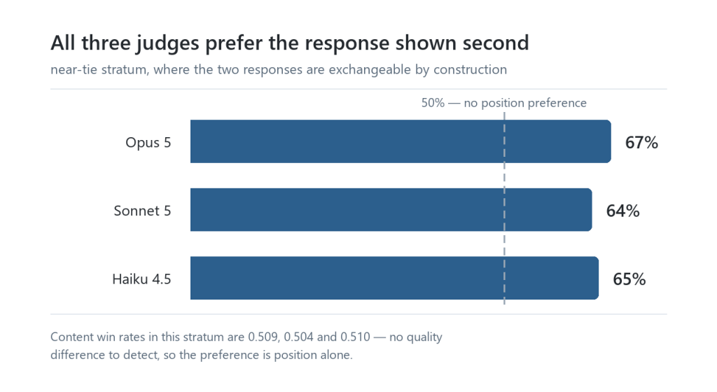
The cleanest measurement comes from the near-tie stratum, where both responses are independent samples from the same model on the same prompt. They are exchangeable by construction, and the data confirms it: the order-balanced content win rate is 0.509, 0.504, and 0.510 across the three judges, all straddling 0.5. There is no quality difference to detect.
| Judge | β (near-tie) | Second position wins |
|---|---|---|
| Opus 5 | −0.173 [−0.203, −0.145] | 67% |
| Sonnet 5 | −0.138 [−0.164, −0.113] | 64% |
| Haiku 4.5 | −0.148 [−0.180, −0.118] | 65% |
Given two responses of equivalent quality, all three judges pick the second one about two thirds of the time. This is recency, and it holds across a wide capability range. Pooled across both strata the effect is smaller, around −0.10, or roughly a 60/40 split.
The published literature finds both directions and reports that the direction is volatile across model families and tasks, so a within-family result like this one should not be read as universal.
A pre-registered check failed, and it matters
The design included a manipulation check: pair a Sonnet 5 response against a Haiku 4.5 response on the same prompt, and the stronger arm should win at least 65% of the time. All three judges failed it, at 0.536, 0.572, and 0.550.
Two explanations fit and this data cannot separate them. Either the judges discriminate poorly, or the two models genuinely produce near-equivalent 150-350 word answers on these prompts. The judges are highly consistent (ICC 0.80 to 0.94), so they are not guessing — but consistency is not discrimination, and a reliable judge can still be reliably indifferent.
What this costs: the stratified interpretation is void, and the pooled estimate mixes one clean stratum with one compromised one. What survives: β itself, which cancels content preference algebraically, and the near-tie result, which never depended on the manipulation working. Reporting this is the point of pre-registering. A criterion that cannot fail is not a criterion.
A token ceiling does not just lose data, it biases what is left
The first run capped judge output at 64 tokens, sized for a one-line verdict. 11.9% of judgments were truncated mid-analysis and lost. Raising the ceiling to 256 changed almost nothing (12.2%). Raising it to 4,096 dropped the failure rate to 0.2%.
The interesting part is what the discarded judgments were. Retrying previously-successful calls at 4,096 agreed with the originals only 89.3% of the time, against a same-ceiling noise floor of 95.6% measured from replicate judging. The difference is −0.063 [−0.107, −0.021], and the equivalence test failed.
max_tokens is a stopping condition, not a generation parameter, so it does not change how the model samples. But a low ceiling censors on output length, and output length correlates with verdict category. The surviving sample is therefore biased with respect to the outcome. Truncation was also not distributed the way verbosity intuition suggests: at the 64-token ceiling, Sonnet 20.7%, Opus 13.8%, Haiku 1.4%. Most evaluation harnesses cap judge output tightly to control cost.
Limitations
One model family, so nothing here speaks to GPT or Gemini judges. One prompt source, skewed technical. Free-text verdict parsing rather than structured outputs, which the runner did not support. And the quality manipulation failed, so the clear-gap stratum measures less than it was designed to.
Working together
I help teams build evaluation infrastructure they can defend: correct inference for their comparisons, power analysis before they spend on a run, judge bias measured rather than assumed, and calibration against human labels so they know their judge is scoring the thing they care about.

